Simple Power Analysis

Scenario

Assume the following:

I will be running a workshop called “Stats is fun” for a small number of participants. Before the workshop I will ask the participants “How enthusiastic are you about statistics?” and give them a scale from 1 to 5. Afterwards, I will ask the same people the same question and compare the responses.

Question

The primary research question is whether the workshop had an impact on the enthusiasm of the participants for statistics.

Of course, as is, this question cannot be directly answered. We must clearly define ‘impact’ and how we hope to measure it.

Framework

We also need to define the framework we will attempt to use to answer the question as there are several options.

For this example we will stick to the classical (frequentist) hypothesis testing framework.

This framework is characterised by the following key components:

1. Assume the world is boring. There is nothing changing and no differences of interest anywhere.
2. Conduct an experiment and observe something.
3. Calculate the probability of observing something at least as interesting as what was observed, under the assumption that everything is boring on the whole (in the bigger picture we call the population). We call this probability a p-value.
4. If the p-value is large we continue to assume that everything is boring. We do not conclude that there is no difference, because that would be wrong, we are quite sure that the population difference is not actually zero. We simply continue to assume no difference as a substitute for the reality that we really can’t tell what the difference is from our experiment due to insufficient evidence either way.
5. On the other hand, if the p-value is small, we conclude that there is evidence against the boring (null) hypothesis and thus that there is evidence of a difference or change from our experiment.

This framework has many severe flaws, far too many to discuss here, and yet in well designed experiments it does what it is meant to do: help us to talk less nonsense!

The real problem with it is how often it is misused and abused. All commonly used statistical hypothesis tests rely on at least two key assumptions:

1. That the sample taken is representative of the population being discussed.
2. That the test being done is the only one of its kind being applied to the data set.

These assumptions are violated far more often than they hold. Only the second one can be partially adjusted for.

Power

The framework as discussed so far is entirely focussed on the sample and the null hypothesis; yet it is the population and the alternative that are of real world interest in most cases.

1. Among otherwise similar tests, a test with more power is preferred, as more power means it is more likely to pick up the differences of interest.
2. In order for failure to reject the null hypothesis to be interesting, we need a test with a lot of power as we need to argue that, ‘had there been a difference then we would have detected it.’ Failing to reject an underpowered test means nothing as it could easily be caused by not collecting a large enough sample.

For a top journal to take your study seriously in many applied fields, you are required to do a power study in advance. Doing it retrospectively will bias the results.

Yet, power studies are often skipped for various reasons, such as the massive effort involved sometimes, and other constraints overriding the desired power.

Power studies are effort because they require you to describe the expected results of the study in extreme detail, and with uncertainty, prior to actually collecting any data.

There is a shortcut a lot of people like to use though: they cite similar studies with similar or smaller sample sizes that achieved significant results. While this is a logical argument, it does not account for publication bias.

Power study procedure

1. Specify the analysis procedure in full detail. 1. Describe how the data will be collected, cleaned, stored, and prepared for analysis. 1. Then describe the model that will be applied, in full mathematical detail, defining all parameters. 1. And lay out how the model fit will be interpreted and conclusions drawn, using definitive rules.
2. Specify the expected values of all the model parameters, including those describing the uncertainty in your expectations. 1. This should be done twice or more: once under the null hypothesis and at least once under the alternative hypothesis.
3. Using the model and the chosen parameter values, simulate a large number of fake data sets.
4. Perform the analysis on each fake data set one at a time and note the conclusion drawn.
5. Report the proportion of times you reached each possible conclusion for each scenario.
6. Repeat the above 3 steps for each of a variety of sample sizes, and connect the dots to obtain power curves.
7. If you do the above 4 steps under the null hypothesis you hope to see low rejection rates but under the alternative hypothesis you hope to see very high rejection rates.

Smoothed version of our example

Suppose we define ‘impact’ as the average difference in scores, then an obvious model is the t-test setup.

However, we would normally be getting responses on a discrete scale, not accurate real numbers. We will use the real numbers first to show the principle.

So, under the alternative I define the model and expected parameters as follows:

\[\begin{aligned} x_i &= \text{ before score for person }i \\ y_i &= \text{ after score for person }i \\ d_i &= y_i - x_i,\ i = 1\dots n \\ d_i &\sim N(\mu_d, \sigma^2_d) \\ \mu_d &= 0.3 \\ \sigma^2_d &= 1 \end{aligned}\]

where the numbers are chosen based on a combination of personal expectation and results from previous studies of a similar kind.

Our decision rule is that the p-value from a t-test comparing the average difference to zero \((H_0:\mu_d=0)\) is less than \(\alpha=0.05\).

The question to be answered first is, “What is the minimum sample size needed to obtain at least 80% power?”

In this simple scenario the question can be quickly answered using one of several power calculation packages in R. We will do it from first principles instead, for illustration and because scenarios can quickly stop being simple.

n_datasets <- 2000
Sample_Size <- seq(10, 150, 10)
sim1 <- \(n, mu_d = 0.3, sigma_d = 1) {
  rnorm(n, mu_d, sigma_d)
}

if (!file.exists("power1.rds")) {
  (Sample_Size |> sapply(\(n) {
    n_datasets |> replicate({
      (n |> 
         sim1() |>
         t.test())$p.value
      })
  }) < 0.05) |> colMeans() -> Power
  Power |> saveRDS("power1.rds")
} else {
  Power <- readRDS("power1.rds")
}

plot(Sample_Size, Power, type = 'l', col = 'purple', lwd = 3)
grid()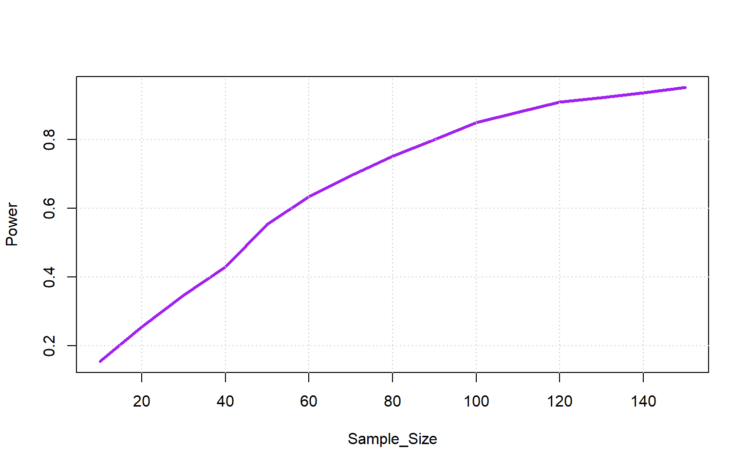

So the optimal sample size is 100.

Two sample versus Paired sample

Let us compare the paired data example above with what happens when the data isn’t matched correctly.

Suppose I forgot to ask each person for a unique identifier, so we still have the same sized samples but no longer paired. To make this a fair comparison, we keep the other factors the same.

To be realistic we incorporate some correlation between the responses for the case where we are able to partially line up the responses.

\[\begin{aligned} x_i &= \text{ before score for person }i \\ y_i &= \text{ after score for person }i \\ [x_i\ y_i] &\sim N_2([3.7\ 4], [1\ \rho; \rho\ 1]) \\ \end{aligned}\]

n_datasets <- 2000
Sample_Size <- seq(50, 250, 20)
sim2 <- \(n, rho = 0.5, mu = c(3.7, 4), sigma = matrix(c(1, rho, rho, 1), 2)) {
  MASS::mvrnorm(n, mu, sigma)
}
rho_seq <- seq(0.1,0.9,0.2)

if (!file.exists("power2.rds")) {
  rho_seq |> sapply(\(rho) {
  (Sample_Size |> sapply(\(n) {
    n_datasets |> replicate({
      n |> sim2(rho) -> d_mat
      t.test(d_mat[,1], d_mat[,2])$p.value
    })
  }) < 0.05) |> colMeans() }) -> Power
  Power |> saveRDS("power2.rds")
} else {
  Power <- readRDS("power2.rds")
}

plot(range(Sample_Size), range(Power), type = 'n', xlab = "Sample Size", ylab = "Power")
grid()
for (i in 1:ncol(Power)) {
  lines(Sample_Size, Power[,i], col = i, lwd = 3)
}
legend('bottomright', legend = rho_seq, title = expression(rho), lwd = 3, col = 1:ncol(Power))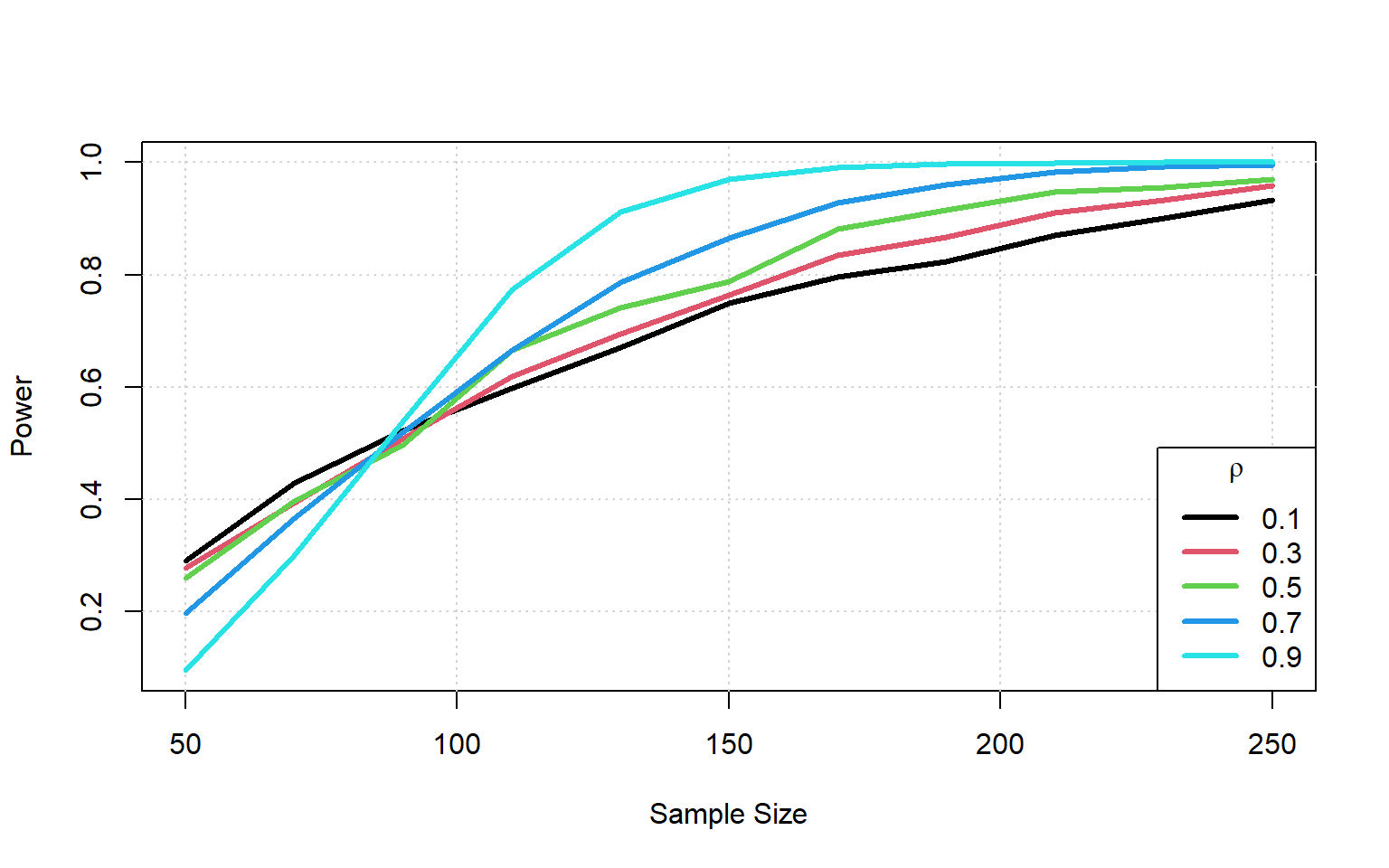

We note that only as the correlation approaches 1 (unrealistic) do we approach the same power we had as with the paired data. Paired data is more powerful.

Unbalanced samples

Suppose now that instead of balanced samples with correlation, we had two independent samples of different sizes. This would occur any time we survey two different groups of people.

\[\begin{aligned} x_i &= \text{ before score for person }i,\ i=1:n_1 \\ y_j &= \text{ after score for person }j,\ j=1:n_2 \\ x_i &\sim N(3.7, 0.9) \\ x_j &\sim N(4, 1.1) \\ \end{aligned}\]

n_datasets <- 2000
Sample_Size <- seq(50, 250, 20)
sim2sample <- \(n1, n2) {
  list(rnorm(n1, 3.7, 0.9), rnorm(n2, 4, 1.1))
}

if (!file.exists("power3.rds")) {
  Sample_Size |> sapply(\(n1) {
  (Sample_Size |> sapply(\(n2) {
    n_datasets |> replicate({
      sim2sample(n1, n2) -> d_list
      t.test(d_list[[1]], d_list[[2]])$p.value
    })
  }) < 0.05) |> colMeans() }) -> Power
  Power |> saveRDS("power3.rds")
} else {
  Power <- readRDS("power3.rds")
}

plot(range(Sample_Size), range(Power), type = 'n', xlab = expression(n[2]), ylab = "Power")
grid()
for (i in 1:ncol(Power)) {
  lines(Sample_Size, Power[,i], col = i, lwd = 3)
}
legend('bottomright', legend = Sample_Size, title = expression(n[1]), lwd = 3, col = 1:ncol(Power))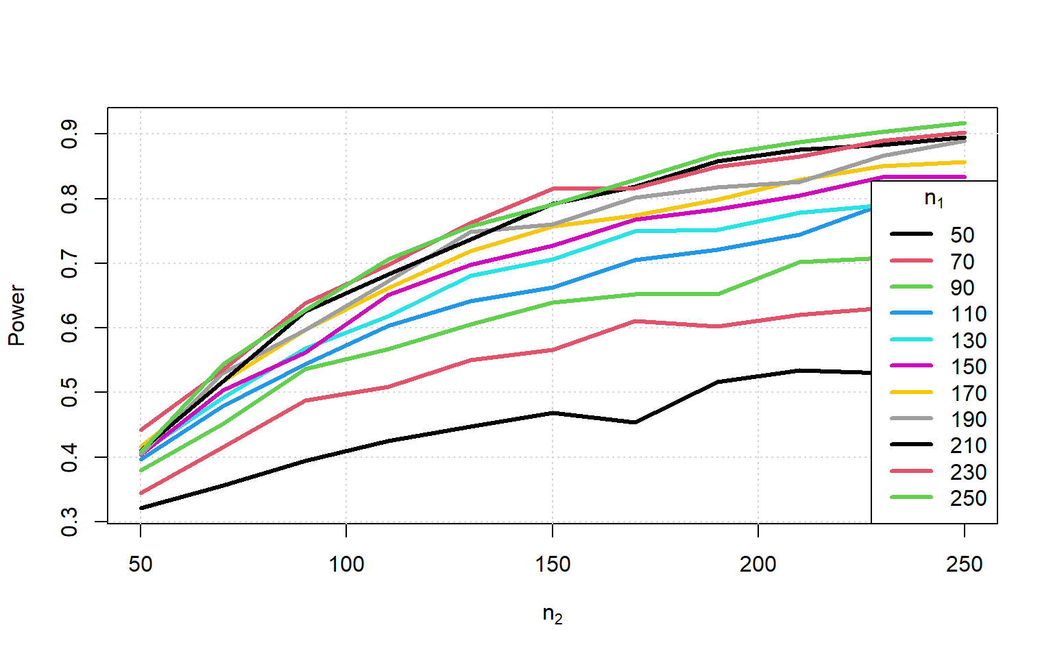

We now see that we need the smaller sample size to be larger than the combined sample size in the paired case to get close to the same power.

Discrete version of our example

We would normally be getting responses on a discrete scale, not accurate real numbers. We will now use discrete numbers are compare to see the impact on power.

So, under the alternative I define the model and expected parameters as follows:

\[\begin{aligned} x_i &= \text{ before score for person }i \\ y_i &= \text{ after score for person }i \\ d_i &= y_i - x_i,\ i = 1\dots n \\ d_i &\sim roundedN(\mu_d, \sigma^2_d) \\ \mu_d &= 0.3 \\ \sigma^2_d &= 1 \end{aligned}\]

where the numbers are chosen based on a combination of personal expectation and results from previous studies of a similar kind.

Our decision rule is that the p-value from a t-test comparing the average difference to zero \((H_0:\mu_d=0)\) is less than \(\alpha=0.05\).

The question to be answered first is, “What is the minimum sample size needed to obtain at least 80% power?”

In this simple scenario the question can be quickly answered using one of several power calculation packages in R. We will do it from first principles instead, for illustration and because scenarios can quickly stop being simple.

n_datasets <- 2000
Sample_Size <- seq(10, 150, 10)
sim1 <- \(n, mu_d = 0.3, sigma_d = 1) {
  rnorm(n, mu_d, sigma_d) |> round()
}

if (!file.exists("power4.rds")) {
  (Sample_Size |> sapply(\(n) {
    n_datasets |> replicate({
      (n |> 
         sim1() |>
         t.test())$p.value
      })
  }) < 0.05) |> colMeans() -> Power
  Power |> saveRDS("power4.rds")
} else {
  Power <- readRDS("power4.rds")
}

plot(Sample_Size, Power, type = 'l', col = 'purple', lwd = 3)
grid()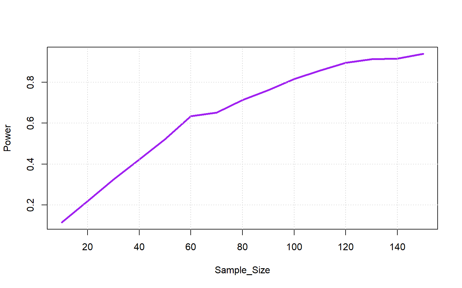

So the optimal sample size is 100.

This is larger than before due to the measurement error.

Unbalanced samples

Suppose now that we had two independent samples of different sizes. This would occur any time we survey two different groups of people.

\[\begin{aligned} x_i &= \text{ before score for person }i,\ i=1:n_1 \\ y_j &= \text{ after score for person }j,\ j=1:n_2 \\ x_i &\sim roundedN(3.7, 0.9) \\ x_j &\sim roundedN(4, 1.1) \\ \end{aligned}\]

n_datasets <- 2000
Sample_Size <- seq(50, 250, 20)
sim2sample <- \(n1, n2) {
  list(round(rnorm(n1, 3.7, 0.9)), round(rnorm(n2, 4, 1.1)))
}

if (!file.exists("power5.rds")) {
  Sample_Size |> sapply(\(n1) {
  (Sample_Size |> sapply(\(n2) {
    n_datasets |> replicate({
      sim2sample(n1, n2) -> d_list
      t.test(d_list[[1]], d_list[[2]])$p.value
    })
  }) < 0.05) |> colMeans() }) -> Power
  Power |> saveRDS("power5.rds")
} else {
  Power <- readRDS("power5.rds")
}

plot(range(Sample_Size), range(Power), type = 'n', xlab = expression(n[2]), ylab = "Power")
grid()
for (i in 1:ncol(Power)) {
  lines(Sample_Size, Power[,i], col = i, lwd = 3)
}
legend('bottomright', legend = Sample_Size, title = expression(n[1]), lwd = 3, col = 1:ncol(Power))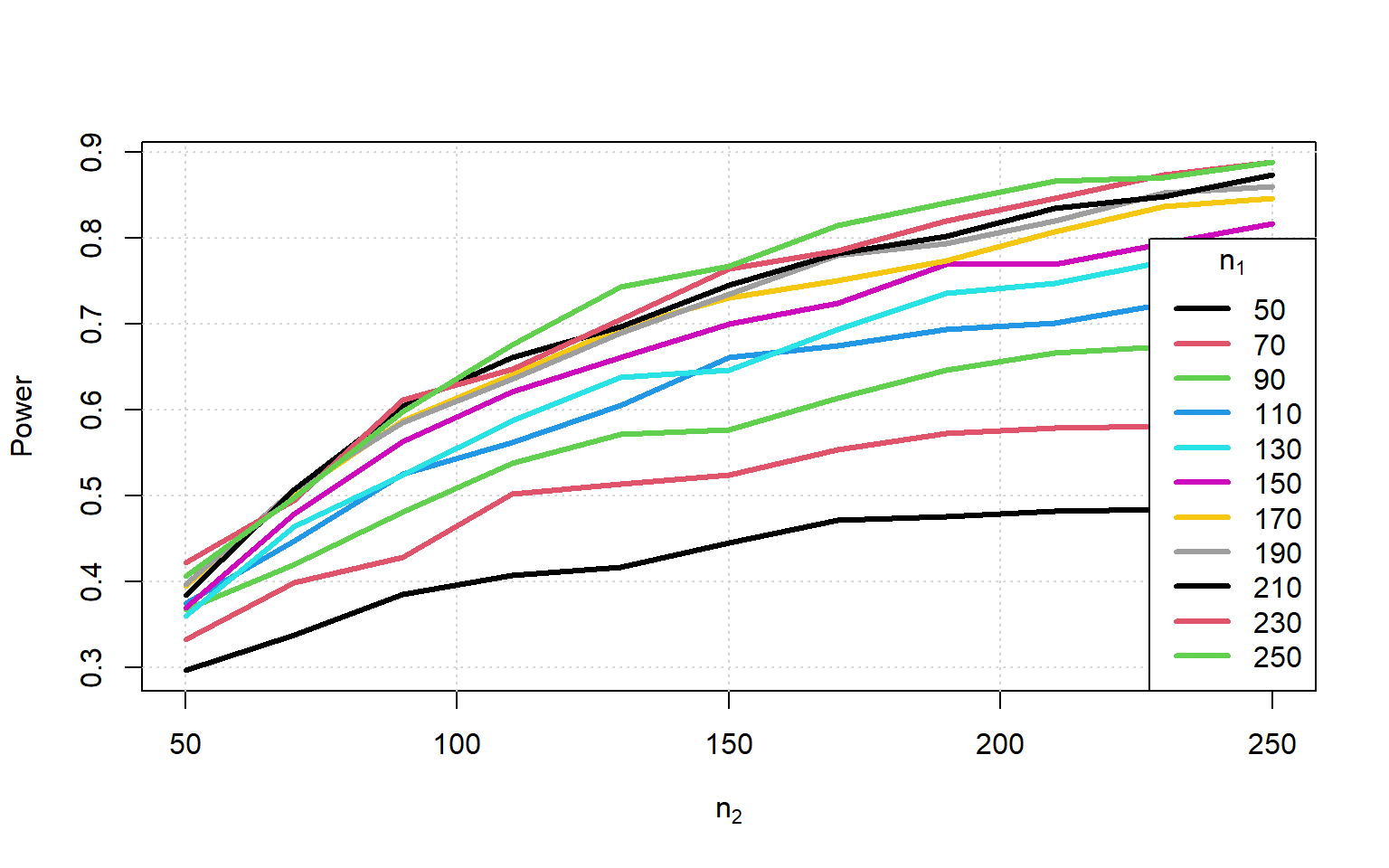

Again we see that the measurement error lowers our power even further.

U test

What if we used the Mann-Whitney test instead of a t-test?

n_datasets <- 2000
Sample_Size <- seq(50, 250, 20)
sim2sample <- \(n1, n2) {
  list(round(rnorm(n1, 3.7, 0.9)), round(rnorm(n2, 4, 1.1)))
}

if (!file.exists("power6.rds")) {
  Sample_Size |> sapply(\(n1) {
  (Sample_Size |> sapply(\(n2) {
    n_datasets |> replicate({
      sim2sample(n1, n2) -> d_list
      wilcox.test(d_list[[1]], d_list[[2]])$p.value
    })
  }) < 0.05) |> colMeans() }) -> Power
  Power |> saveRDS("power6.rds")
} else {
  Power <- readRDS("power6.rds")
}

plot(range(Sample_Size), range(Power), type = 'n', xlab = expression(n[2]), ylab = "Power")
grid()
for (i in 1:ncol(Power)) {
  lines(Sample_Size, Power[,i], col = i, lwd = 3)
}
legend('bottomright', legend = Sample_Size, title = expression(n[1]), lwd = 3, col = 1:ncol(Power))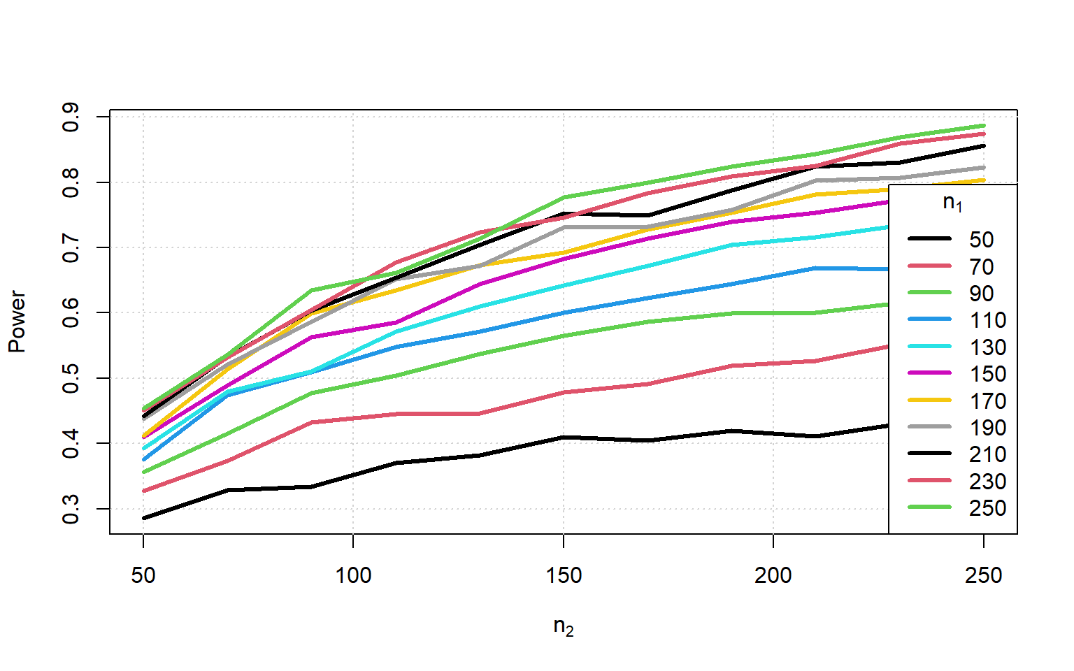

There appears to be only a tiny drop in power in spite of the change in hypothesis.

Regression

Suppose now that we want to test whether gender has an effect on the change in enthusiasm, while simultaneously still assessing whether the change is meaningful in the first place. We could try the following model:

\[\begin{aligned} x_i &= \text{ before score for person }i \\ y_i &= \text{ after score for person }i \\ d_i &= y_i - x_i,\ i = 1\dots n \\ d_i &\sim roundedN(\mu_{d_i}, \sigma^2_d) \\ \end{aligned}\]

But now we assume the following relationship, where \(g_i\) is a gender indicator variable with a value of 1 for female participants:

\[\begin{aligned} \mu_{d_i} &= 0.3 + 0.4g_i \\ \sigma^2_d &= 1 \end{aligned}\]

We now have two power curves and are interested in the lowest one.

n_datasets <- 2000
Sample_Size <- seq(50, 250, 20)
simreg <- \(n) {
  rnorm(n, 0.3 + 0.4*round(seq_len(n)/(n+1)), 1) |> round()
}

if (!file.exists("power7.rds")) {
  (Sample_Size |> sapply(\(n) {
    n_datasets |> replicate({
      y <- simreg(n)
      g <- round(seq_len(n)/(n+1))
      res <- coef(summary(lm(y ~ g)))
      res[,4] < 0.05
      }) |> matrix(ncol = 2, byrow = TRUE) |> colMeans()
  })) |> t() -> Power
  Power |> saveRDS("power7.rds")
} else {
  Power <- readRDS("power7.rds")
}

plot(range(Sample_Size), range(Power), type = 'n', xlab = expression(n[2]), ylab = "Power")
grid()
for (i in 1:ncol(Power)) {
  lines(Sample_Size, Power[,i], col = i, lwd = 3)
}
legend('bottomright', legend = c("Male vs 0", "Female vs Male"), title = "Effect", lwd = 3, col = 1:ncol(Power))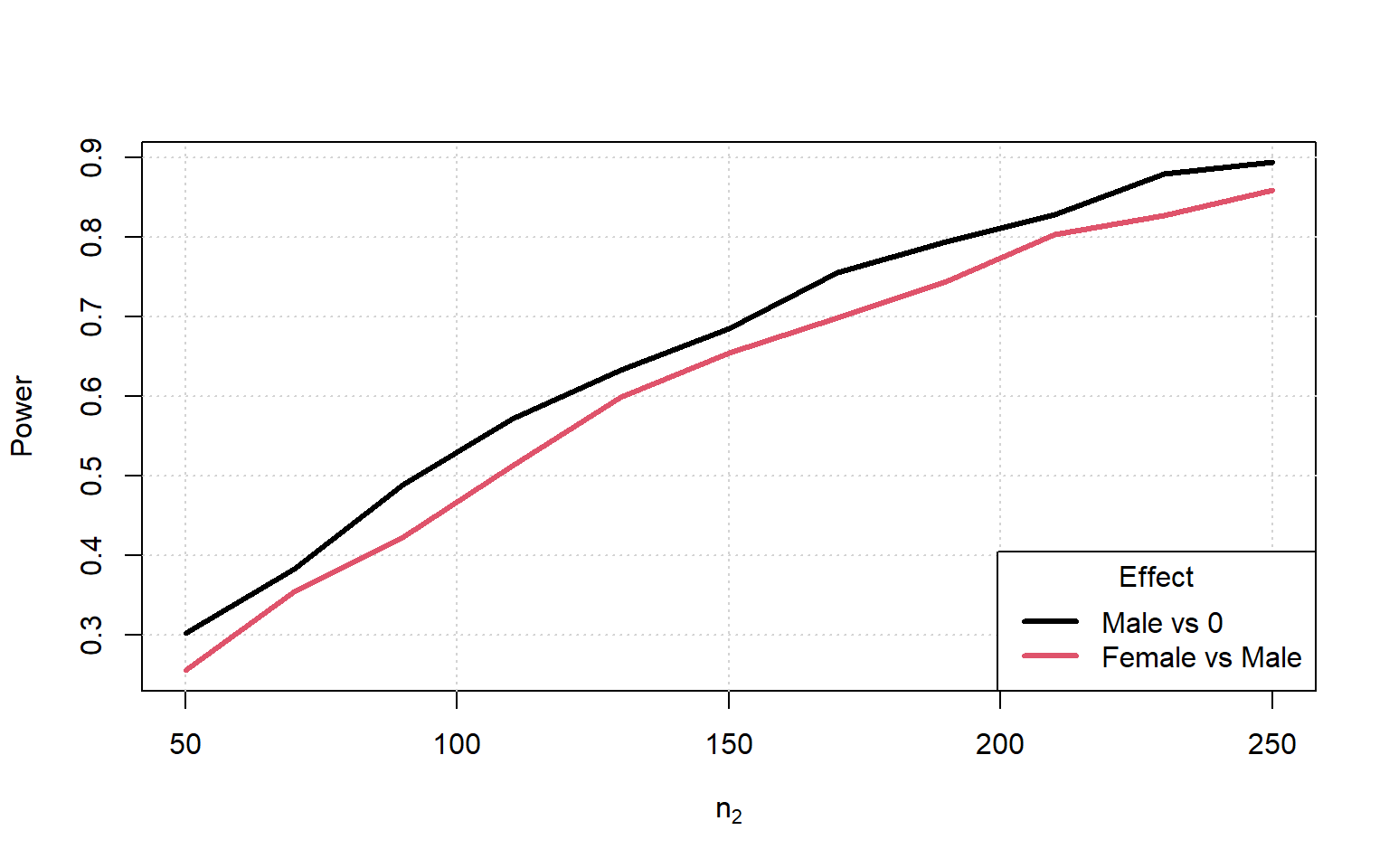

Conclusion

While the above models are all quite simple, the principles demonstrate translate to models of higher complexity. As long as you can follow the core steps then you can estimate power or required sample size.

Steps:

1. Write down the model mathematically,
2. specify expected values for all parameters,
3. simulate data sets,
4. fit the model to each data set as if the parameters are unknown,
5. calculate the values (usually p-values) of interest,
6. summarise the results and interpret.