Robust biplots

Motivation

Biplots can contain a lot of information. In a previous post called Drawing an interactive biplot with echarts4r we saw how to move from a static biplot, drawn with biplotEZ, to an interactive biplot, drawn with echarts4r.

Still, those of you with a keen eye would have seen that two of the variables were illustrated essentially on top of one another. In an interactive plot it is sometimes possible to still separate them visually but this is a general problem that occurs when drawing biplots.

Ideally, biplots should be drawn deliberately one at a time, with care and attention to data preparation. However, practically one often might need to draw many biplots in a loop and the hope is to have them come out as interpretable automatically.

When drawing multiple biplots as part of an automated, looping, or otherwise recurring, process it is important to have a robust pipeline.

Robust solution: plot with accompanying tables

Normally the goal with a biplot is to place a lot of information on a single figure. However, a single figure can only hold so much information, and when that information overlaps on the figure then there is not a lot we can do.

If we allow for additional information to accompany the figure then there is much that can be done to improve on the figure itself.

I envision two additional steps:

1. Pre-processing of input data for severe data problems,
2. Post-processing of PCA output to avoid visual problems,

with the results of these combined into a small table to accompany the biplot.

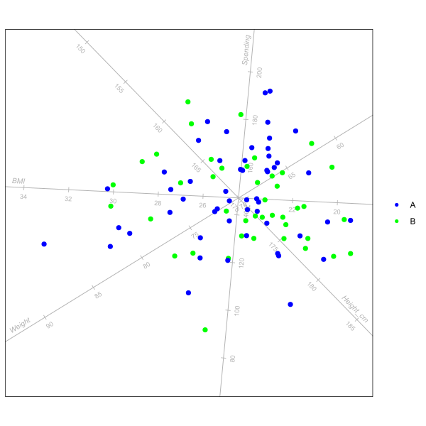
data_check <- function(df, threshold = 0.97, display_issues = TRUE) {
  if (!any(class(df) %in% "data.frame")) {df <- as.data.frame(df)}
  varnames <- names(df)
  num_vars <- seq_len(ncol(df)) |> sapply(\(j) {
    isnum <- is.numeric(df[[j]])
  })
  valid_vars <- seq_len(ncol(df)) |> sapply(\(j) {
    if (num_vars[j]) {
      sd(df[[j]]) > 0
    } else {
      FALSE
    }
  })
  degenerate <- num_vars & !valid_vars
  if (any(degenerate)) {
    degen_df <<- data.frame(Name = varnames[degenerate], 
                            Number = which(degenerate), 
                            Problem = "Degenerate"
                           )
    if (display_issues) {
      cat("\n\nThe following variables have no variation to model:\n\n")
      degen_df |> knitr::kable() |> print()
      cat("\n\n")
    }
  }
  numv <- which(valid_vars)
  num_df <- df[,valid_vars]
  p <- ncol(num_df)
  abscormat <- abs(cor(num_df) - diag(p))
  colinear_df <<- seq(1, p - 1) |> lapply(\(i) {
    seq(i + 1, p) |> lapply(\(j) {
      if (abscormat[i,j] > threshold) {
        m <- lm(df[[numv[j]]] ~ df[[numv[i]]]) |> coef()
        data.frame(Num1 = numv[i], Num2 = numv[j], 
                   Var1 = varnames[numv[i]], 
                   Var2 = varnames[numv[j]], 
                   Corr = abscormat[i,j],
                   Formula = paste0(
          varnames[numv[j]], " ≈ ", round(m[2], 3), "*", varnames[numv[i]], 
          " + ", round(m[1], 3)))
      }
    }) |> do.call(rbind, args = _)
  }) |> do.call(rbind, args = _)
  if (display_issues && !is.null(colinear_df)) {
    cat("\n\nThe following variables have severe colinearity:\n\n")
    colinear_df[,3:6] |> knitr::kable() |> print()
    cat("\n\n")
  }
  all_fine <- !degenerate
  if (!is.null(colinear_df)) {all_fine[colinear_df$Num1] <- FALSE}
  df[, all_fine]
}

missing_check <- function(df, threshold = 0.5, display_issues = TRUE) {
  empty_vars <- seq_len(ncol(df)) |> sapply(\(j) {
    mean(is.na(df[[j]])) > threshold
  })
  if (display_issues & any(empty_vars)) {
    cat("\n\nVariables dropped for containing too few non-missing values:\n\n", 
        paste(names(df)[empty_vars], collapse = ", "), ".", sep = "")
  }
  df <- df[, !empty_vars]
  num_vars <- seq_len(ncol(df)) |> sapply(\(j) {
    isnum <- is.numeric(df[[j]])
  })
  problem_rows <- seq_len(nrow(df)) |> sapply(\(r) {
    any(is.na(df[r, num_vars]))
  })
  if (display_issues & any(problem_rows)) {
    cat("\n\nRows dropped for containing missing values:\n\n", 
        paste(which(problem_rows), collapse = ", "), ".", sep = "")
  }
  df[!problem_rows, ]
}

good_angles <- function(bp, threshold = 0.07, display_issues = TRUE) {
  angles <- atan2(bp$ax.one.unit[,2], bp$ax.one.unit[,1]) %% pi
  dist_df <- rbind(data.frame(Varnum = 1, Fine = TRUE, Closest = 1), 
    seq(2, length(angles)) |> lapply(\(i) {
    difs <- abs(angles[seq_len(i-1)] - angles[i])
    data.frame(
      Varnum = i, 
      Fine = all(difs > threshold), 
      Closest = which.min(difs)
    )
  }) |> do.call(rbind, args = _))
  bp$axes_angles <- dist_df
  if (!all(dist_df$Fine)) {
    issues_df <- dist_df |> subset(!Fine)
    issues_df$Closest_varname <- bp$axes$names[issues_df$Closest]
    varnames <- colnames(bp$X)
    issues_df$Formula <- seq_len(nrow(issues_df)) |> sapply(\(j) {
      m <- lm(bp$X[,issues_df$Varnum[j]] ~ bp$X[,issues_df$Closest[j]]) |> 
        coef()
      paste0(varnames[issues_df$Varnum[j]], " ≈ ", round(m[2], 3), 
             "*", varnames[issues_df$Closest[j]], 
            " + ", round(m[1], 3))
    })
    if (display_issues) {
      issues_df |> kable() |> print()
    }
    bp$angle_issues_df <- issues_df
  }
  bp$good_angles <- dist_df$Fine |> which()
  bp
}

robust_biplot <- function(df, group_col = 1, compile_issues = TRUE) {
  clean_df <- df |> missing_check(display_issues = FALSE) |> 
    data_check(display_issues = FALSE)
  bp_obj <- clean_df |> biplot(classes = clean_df[[group_col]],
                               scaled = TRUE) |> PCA() |> 
    good_angles(display_issues = FALSE)
  prop_explained <- bp_obj$eigenvalues[1:2]/sum(bp_obj$eigenvalues)
  p_expl <- round(prop_explained*100)
  plt <- bp_obj |> 
    axes(which = bp_obj$good_angles) |> 
    plot()
  if (compile_issues) {
    tryCatch({
      cat("\n\n")
      degen_df |> kable() |> print()
    }, error = \(e) NULL)
    tryCatch({
      cat("\n\n")
      colinear_df |> kable() |> print()
    }, error = \(e) NULL)
    tryCatch({
      cat("\n\n")
      bp_obj$angle_issues_df |> kable() |> print()
    }, error = \(e) NULL)
  }
  # library(ggplot2)
  # plt + labs(x = paste0("PCA (", p_expl[1], "%)"), 
  #                    y = paste0("PCA (", p_expl[2], "%)"))
  bp_obj |> invisible()
}

Example

Consider this horrific data set:

set.seed(123)
test_n <- 100
test_df <- data.frame(
  Group = sample(LETTERS[1:2], test_n, TRUE), 
  Height = rnorm(test_n, 1.7, 0.06) |> round(2),
  Weight = rnorm(test_n, 70, 6) |> round(1),
  Intercept = rep(1, test_n), 
  Note = c("This is a made up data set", rep(NA_character_, test_n - 1)),
  Spending = sample(100:200, test_n, TRUE),
  `Extra unrelated variable with a rediculously long name` = rbinom(test_n, 100, 0.4)
)
test_df$BMI <- test_df$Weight/test_df$Height^2
test_df$Height_cm <- test_df$Height*100
test_df$Spending[sample(seq_len(test_n), 5)] <- NA_integer_

table.dataTable tbody td {
  font-size: 16px;
  padding: 6px 10px;
}

library(DT)
datatable(test_df, rownames = FALSE, filter = "top", 
          options = list(pageLength = 10, dom = "tp"))

And the one line generic solution:

test_df |> robust_biplot("Group")

Name	Number	Problem
Intercept	4	Degenerate

Num1	Num2	Var1	Var2	Corr	Formula
2	8	Height	Height_cm	1	Height_cm ≈ 100*Height + 0

	Varnum	Fine	Closest	Formula
3	3	FALSE	2	Extra.unrelated.variable.with.a.rediculously.long.name ≈ -0.092*Spending + 0